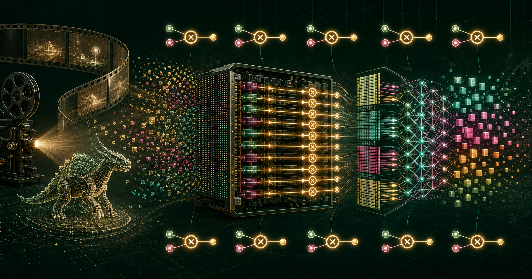
Programmable Appearance Came First
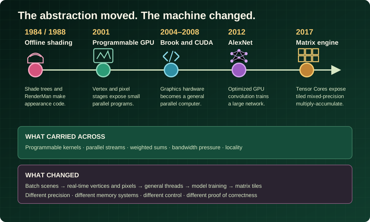
Rob Cook's 1984 "shade trees" composed surface and lighting behavior from programmable operations. Pixar's 1988 RenderMan Interface carried that idea into a full shading language. NVIDIA's GeForce3 introduced a user-programmable consumer vertex engine in 2001.
The path runs through workload and programming model: film requirements shaped a scalable renderer and language; real-time shading research translated the model; stream-computing research opened the GPU; neural networks exploited the resulting parallel machine.
Movie Images Forced A New Scale
In the early 1980s, Ed Catmull, Loren Carpenter, and Rob Cook at Lucasfilm sought computer-generated images that could sit beside live-action photography without jagged edges, polygonal surfaces, absent motion blur, or crude materials.
The REYES planning target called for 5 million pixels, 80 million micropolygons per image, 16 samples per pixel, and about 300 floating-point operations per micropolygon. That scale demanded a new architecture.
The bucket, split, dice, shade, hide, filter, display pipeline kept working sets compact, exploited locality, and shaded coherent vectorizable grids. Sampling, visibility, texture access, caching, and geometry order mattered alongside floating-point throughput.
Turning appearance into code gave technical directors a programmable language for surfaces, lights, deformations, and volumes instead of a growing collection of fixed material switches.
Offline And Interactive Graphics Chose Different Interfaces
Pixar and Silicon Graphics explored a common procedural 3D interface in 1987, then followed the abstractions their workloads required.
RenderMan described complete scenes for batch photorealistic rendering over hours. SGI's interactive systems emphasized lower-level drawing commands, immediate response, z-buffers, accumulation buffers, 2D applications, and graphical interfaces.
The pipelines diverged while programmable shading crossed between them as the enduring idea.
The Programming Model Reached The GPU
Pat Hanrahan's Stanford group developed the real-time shading language RTSL. Hanrahan and Catmull's 2021 retrospective traces its influence through NVIDIA Cg, Microsoft HLSL, and GLSL. In the same research lineage, Ian Buck developed Brook for GPUs; Brook evolved into CUDA.
GeForce3's 2001 vertex engine placed a user-programmable instruction stream inside a tightly tuned graphics stage. Programs operated on independent vertices, letting the machine preserve transparent multithreading and parallel throughput while accepting new code.
Unified-shader designs let more graphics stages share a parallel processor array. CUDA exposed threads, memory, and synchronization directly, opening the same throughput machine to computation beyond the raster pipeline.
One Arithmetic Motif Drives Four Hardware Forms
Graphics and learning both repeat weighted sums:
accumulator = accumulator + value * weightA lighting calculation forms dot products between directions, then combines the results with colors and material terms. A convolution forms dot products between an image neighborhood and a learned kernel. A dense neural layer multiplies an input vector by many weight vectors. Matrix multiplication performs many dot products together.
The recurring operation connects the workloads, while each instruction defines a distinct numerical and hardware contract.
a × b + c with one final rounding. Fermi introduced IEEE-754-2008-style FP32 FMA and implemented FMA for both FP32 and FP64; GT200 already supported FP64 FMA. Earlier single-precision GPU MAD instructions used a different numerical contract.AlexNet Turned GPU Throughput Into A Training Advantage
The 2012 AlexNet team paired current GPUs with a highly optimized implementation of two-dimensional convolution to train an unusually large convolutional network on high-resolution images.
The network used five convolutional and three fully connected layers. Training took five to six days on two 3 GB GTX 580 GPUs. The team split the model across both devices to fit memory and connected them only at selected layers, keeping communication a tolerable fraction of computation.
The paper forecast the next step directly: faster GPUs, more memory, and larger datasets could support larger models and improve results.
Convolution and dense layers expose vast fields of similar dot products. That arithmetic density gave a throughput-oriented parallel machine useful work at every lane.
The Scalar Loop Became a Matrix Tile
By 2017, NVIDIA's Volta Tensor Cores exposed D = A × B + C on matrix tiles. The first generation accepted FP16 multiplication inputs with FP16 or FP32 accumulation. NVIDIA counted 64 mixed-precision floating-point FMA operations per Tensor Core per clock.
The instruction shape, cooperating threads, data layout, precision contract, and accumulation behavior all changed. A recurring sum of products had become a dedicated matrix datapath.
A scalar FP32 FMA rate, an early shader MAD rate, and mixed-precision Tensor TFLOPS describe different numerical contracts. The architecture tells the larger story: the hardware unit grew to match the dominant workload.
Each Workload Reshapes The Machine
Rendering organizes a complete image pipeline. REYES joined geometry splitting and dicing with stochastic sampling, visibility, texture access, locality, and bounded working sets. Modern path tracing adds ray traversal, divergent paths, complex shaders, random sampling, and large scene data.
Training organizes a complete learning pipeline. Data loading, activation functions, normalization, softmax, optimizer state, memory movement, and communication across accelerators all compete with matrix arithmetic for time and bandwidth.
Precision belongs to the design. A visually acceptable rendering error, an IEEE scientific result, and a stable mixed-precision training step demand different tolerances. Low-precision training coordinates numerical range, accumulation, scaling, and parameter updates.
The documented connection runs through programming models, workload fit, and increasingly specialized arithmetic. That path explains how programmable appearance helped open a mass-market parallel machine for matrix-scale learning.
Run The Same Ideas At Human Scale
Three working systems bring the graphics-to-silicon path within reach:
- Cheap Pixelless Textures With 2D SDFs pairs a procedural image with the Python, NumPy, and Pillow renderer that produced it.
- Four-Layer Transformer Trained On A CPU exposes the model shape, command, loss record, generated samples, and complete source.
- FMA From RTL To GDSII carries
a × b + cthrough alignment, partial products, normalization, rounding, exceptions, pipeline staging, timing, verification, and layout.
Together they connect image construction, model training, arithmetic architecture, and manufactured silicon.
Workloads Pull Hardware Toward Their Inner Loops
A workload shapes hardware when four things line up: an operation repeats often enough, its dataflow exposes parallel work, a programming interface lets people express new uses, and a large enough market rewards specialized implementation.
Movie rendering helped make programmable appearance a production requirement. Games and real-time graphics made programmable parallel arithmetic a mass-market product. GPU computing opened the machine beyond the raster pipeline. Deep learning arrived with dot-product-heavy work large enough to justify matrix-specific, mixed-precision hardware.
The movie frame and the model token apply the same pressure: keep enormous streams of arithmetic fed. That pressure turns useful abstractions into languages, processors, and dedicated datapaths.
Primary Sources
- Pat Hanrahan and Edwin Catmull, The Design of RenderMan, IEEE Computer Graphics and Applications, 2021.
- Pixar RenderMan, The Evolution of RenderMan.
- Erik Lindholm, Mark Kilgard, and Henry Moreton, A User-Programmable Vertex Engine, SIGGRAPH 2001.
- Ian Buck et al., Scalable Parallel Programming with CUDA, 2008.
- NVIDIA, NVIDIA's Next Generation CUDA Compute Architecture: Fermi, 2009.
- Alex Krizhevsky, Ilya Sutskever, and Geoffrey Hinton, ImageNet Classification with Deep Convolutional Neural Networks, 2012.
- NVIDIA, Programming Tensor Cores in CUDA 9, 2017.
- NVIDIA, Matrix Multiplication Background User's Guide.